1. 논문 소개
'ImageNet Classification with Deep Convolutional Neural Networks'
Alex Krizhevsky, Ilya Sutskever, Geoffrey E. Hinton (NIPS 2012)
(1) Abstract
- ILSVRC(ImageNet Large-Scale Visual Recognition Challenge)-2010 : 120만 개의 고해상도 이미지를 1000개의 서로 다른 class로 분류하는 대회
- 테스트 데이터에서 top-1, top-5 error rates가 각각 37.5%, 17.0%를 기록하며, 기존의 sota보다 훨씬 우수한 결과를 얻었다.
(top-5 error rate란 모델이 예측한 최상위 5개 범주 가운데 정답이 없는 경우의 오류율이다.)
- 6,000만 개의 파라미터, 65만 개의 뉴런으로 신경망을 구성하였으며, 5개의 convolutional layers, 그 중에서 일부는 max pooling layer를 가진다. 마지막에 1000-way softmax fully connected layers 3개로 구성되어 있다.
- 훈련 속도를 높이기 위해 non-saturating neurons를 사용하였으며, GPU로 구현하였다.
- Fully connected layers에서 overfitting을 줄이기 위해 'Dropout'이라는 정규화 방법을 사용하였고, 이는 매우 효과적이었다.
- Dropout을 적용한 모델은 ILSVRC-2012 대회에서 top-5 test error rate를 15.3%를 달성하였는데, 이는 2위 error rate인 26.2%와의 간격이 매우 큰 결과이다.

(2) Introduction
- 현재 object recognition에서는 machine learning 방법을 많이 사용하고 있다. 이러한 object recognition 성능을 높이기 위해서는 1) larger dataset이 필요하며, 2) more powerful model을 학습시키고, 3) overfitting을 방지하기 위한 기술을 사용해야 한다.
- 이전까지의 label의 개수는 그래봤자 10개 남짓이었다. 이러한 simple recognition task에서는 적은 양의 데이터셋과 label-preserving transformation을 통한 augmentation으로도 충분한 인간 정도의 성능을 보였다.
- 대규모 데이터셋 (수백만 장의 이미지와 수천개의 objects)을 학습하기 위한 모델로, CNN을 제안한다.
standard feedforward neural networks에 비교했을 때, connections, parameters가 적기 때문에 훈련이 더 쉽다.
- CNN의 장점에도 불구하고, high resolution (고해상도) images에 대규모로 적용하기에는 비용이 많이 든다.
따라서, 'highly-optimized GPU implementation of 2D convolution'를 활용하여 매우 큰 deep learning CNN을 학습할 수 있도록 한다.
- 5개의 convolutional, 3개의 fully-connected layers를 가지고 있다. (이 중 하나의 레이어만 제거하더라도 떨어지는 성능이 나온다.)
(3) The Dataset
1) ImageNet
- 1,500만 장의 labeled high-resolution images
- 약 22,000개의 카테고리
2) ILSVRC (실제 사용한 데이터셋)
- ImageNet의 subset을 데이터셋으로 사용
- 각 카테고리 별로 1,000개의 이미지가 포함된 총 1,000개의 카테고리
- 약 120만 장의 training images + 5만 장의 validation images + 15만 장의 testing images
3) 데이터 전처리
- ImageNet은 variable-resolution images로 구성되어 있음 (각 이미지 별로 해상도 차이가 있음)
: 일정한 입력 차원을 받기 위해서 256 x 256의 fixed resolution으로 down-sampling 진행
- 각각의 픽셀에서 training set의 평균값을 빼어 centered raw RGB 값으로 모델 학습
(4) The architecture
1) ReLU Nonlinearity
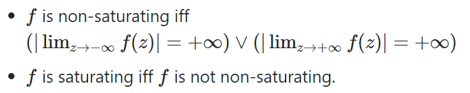
- 일반적으로 tanh, sigmoid를 활성화 함수로 사용했었는데, gradient descent에서의 saturating 문제로 ReLU를 처음 사용하였음
- tanh에서는 출력값이 [-1, 1] 범위에서 존재하여, 논문에서 말하는 'saturating' 상태가 된다.
입력값이 ∞ 또는 -∞가 될수록 기울기가 0에 가까워져 weight 학습이 잘 되지 않는다.
- 반면, ReLU는 [0, ∞] 범위에서 존재하여, non-saturating 함수이다.
입력값이 ∞이더라도 기울기가 0이 아니라 빠르게 수렴된다.
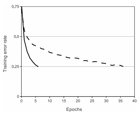
- 실선은 ReLU를 사용했을 때, 점선은 tanh를 사용했을 때 25%의 error rate에 도달하기까지의 epoch을 나타낸 그래프이다.
확실히 실선인 ReLU가 더 빠른 속도로 도달했음을 확인할 수 있다.
2) Training on Multiple GPUs
- GPU 한 개로는 모델의 최대 크기에 제한이 있기 때문에, 모델을 두 개의 GPU로 나눠준다.
- host machine memory 없이도 GPU 간의 메모리에서 직접 read, write가 가능하다.
- 병렬 GPU은 기본적으로 kernel의 절반을 각 GPU에 배치하고, 특정 layer에서만 communicate한다.
(layer 3는 두 GPU에서 모든 커널을 입력 받고, layer 4는 본인 GPU에서만 입력을 받음)
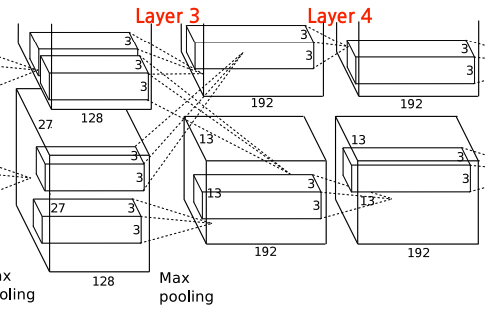
- 교차 검증을 통해 GPU 연결 패턴을 결정한다.
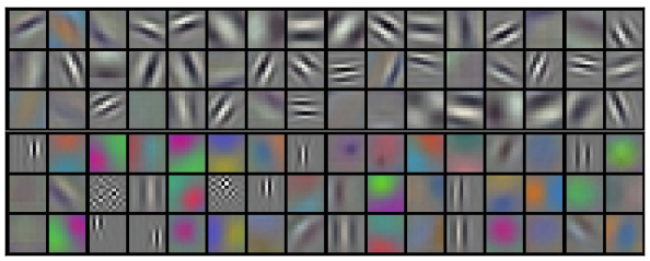
- 224 x 224 x 3 이미지를 kernel size=11로 학습하여 나온 결과인 96개의 결과이다.
위쪽의 48개의 결과는 GPU1, 아래쪽의 48개의 결과는 GPU2로 학습된 결과이다.
GPU1은 색상보다는 형태에, GPU2는 색상과 관련된 피처를 학습하고 있다는, 즉 독립적으로 학습한다는 것을 보여준다.
3) Local Response Normalization
- Local Response Normalization을 통해 generalization을 더 높인다. (현재는 Batch Normalization)
- ReLU를 활성화 함수로 사용했을 때, 양수 입력에 대해서는 그대로 내보내지만 음수 입력에 대해서는 0을 내보낸다.
이렇게 되면, 그 다음 계층에 큰 값이 전달되고, 주변의 작은 값들은 덜 전달되어 학습이 잘 이뤄지지 않는다.
- 이런 현상을 방지하기 위해 LRN이 사용되었다.
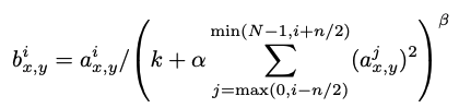
- aix,y : 픽셀 (x, y)에 커널 i를 적용한 결과
- bix,y : LRN 결과
- i : 현재 kernel
- N : 총 kernel 개수
- n : 이웃한 normalization 크기
n개의 이웃한 필터에서의 (x,y)의 결과를 제곱하여 더하면,
값이 클수록 원래 값보다 작게 만들어주고, 작을수록 원래 값보다 크게 만들어주는 normalization 작업인 것이다.
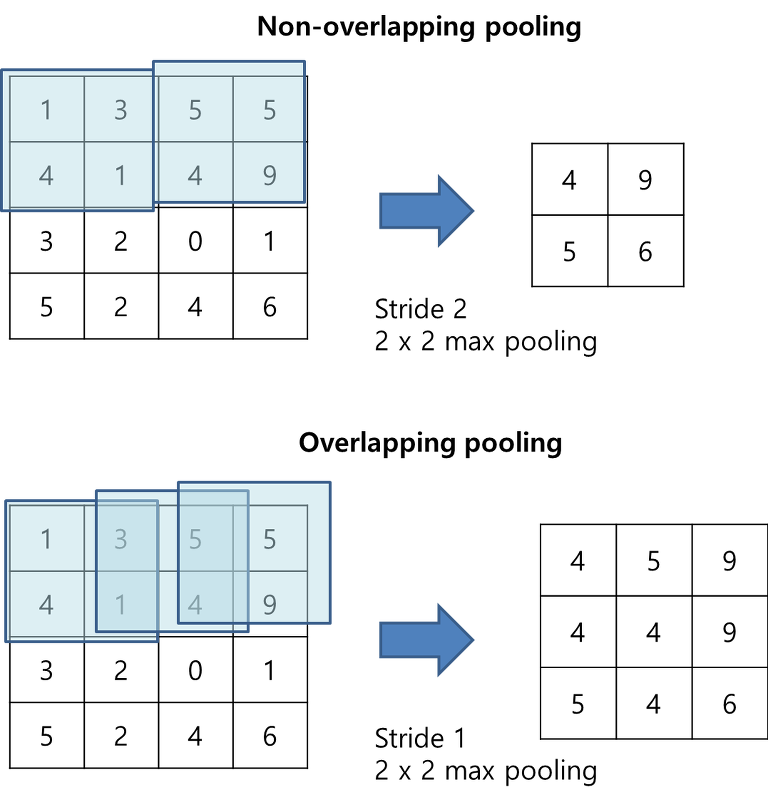
4) Overlapping Pooling
- 일반적으로 pooling은 겹치지 않게 하지만, AlexNet에서는 overlapping 해주었다.
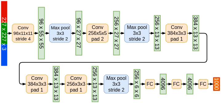
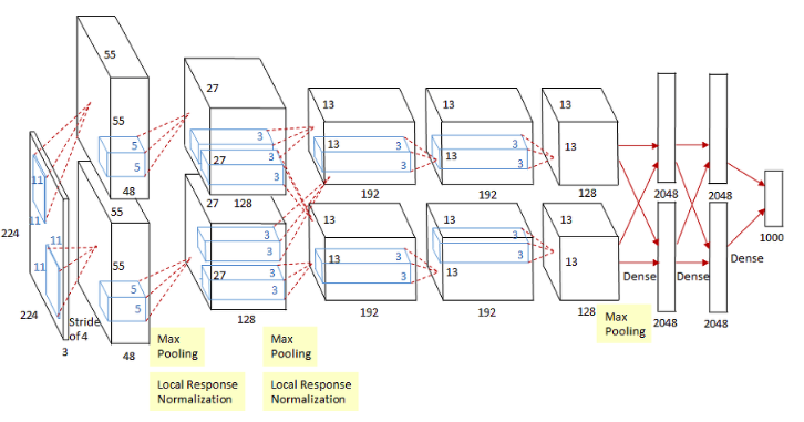
5) Overall Architecture
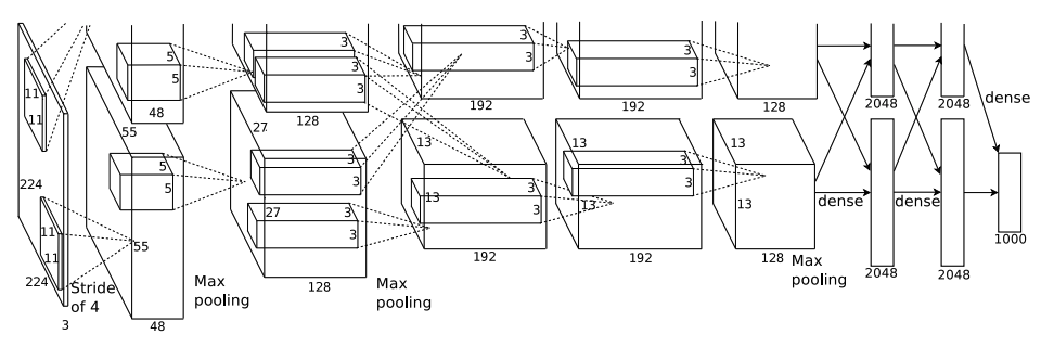
- 5개의 convolutional layers + 3개의 fully connected layers (1000-way softmax)
[ Input layer - Conv1 - MaxPool1 - Norm1 - Conv2 - MaxPool2 - Norm2 - Conv3 - Conv4 - Conv5 - MaxPool3 - FC1 - FC2 - Output layer ]
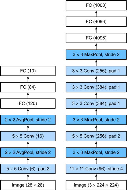
왼쪽은 가장 초기의 CNN 모델인 LeNet-5이며, 오른쪽은 AlexNet이다.
훨씬 더 복잡하고 커진 것을 알 수 있다.
(나중에 사람들이 다시 계산해보니 input layer에서 224 x 224가 아니라 227 x 227이 맞는 크기였다.)
(5) Reducing Overfitting
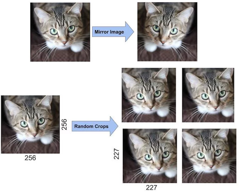
1) Data Augmentation
- overfitting을 막을 수 있는 가장 쉬운 방법은 label-preserving transformation을 활용한 dataset 확장이다.
- 본 논문에서 사용한 data augmentation 방법으로는 다음 두 가지가 있다.
: horizontal reflections (수평 반전), PCA를 활용한 RGB 픽셀 값 변화
- horizontal reflections
- PCA 활용한 RGB 픽셀값 변경
: 각 RGB 이미지 픽셀 벡터 [IRxy,IGxy,IBxy]에 대해서, 모든 이미지 픽셀에 대해 공분산 행렬을 계산한다.
고유값 λi은 RGB 공간의 주성분을 나타내고, 고유벡터 pi은 각 성분의 분산을 나타낸다.
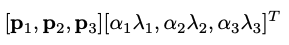
각 픽셀에 위의 값을 더해서, 주성분 방향으로 픽셀 값을 랜덤하게 변형한다.
2) Dropout
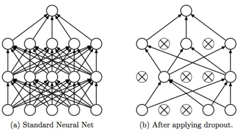
- 확률 0.5로 특정 hidden neuron의 출력값을 0으로 만들어준다.
- 순전파, 역전파 전달이 되지 않으므로 입력이 주어질 때마다 다른 아키텍처를 샘플링하는 것과 동일한 효과를 낸다. 즉, 여러 모델이 가중치를 학습하는 앙상블과 동일한 것이다!
(6) Results
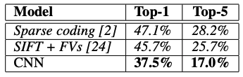
- ILSVRC2010 test set의 Top-1 error rate, Top-5 error rate 결과이다.
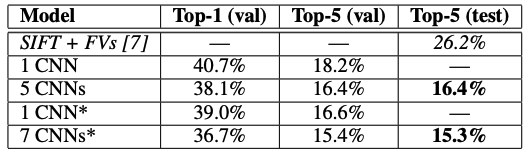
- ILSVRC-2012 validation and test sets에서의 Top-1 error rate, Top-5 error rate 결과이다.
(*는 2011 ImageNet으로 pretrained model)
2. Summary
- Activation 함수로 ReLU 함수를 첫 사용
- MaxPooling 으로 Pooling 적용 및 Overlapping Pooling 적용
- Local Response Normalization (LRN) 사용
- Overfitting을 개선하기 위해서 Drop out Layer와 Weight의 Decay 기법 적용
- Data Augmentation 적용 (좌우 반전, Crop, PCA 변환 등)
- 11x11, 5x5 사이즈의 큰 사이즈의 Kernel 적용. 이후 3x3 Kernel을 3번 이어서 적용
- Receptive Field가 큰 사이즈를 초기 Feature map에 적용하는 것이 보다 많은 feature 정보를 만드는데 효율적이라고 판단
- 하지만 많은 weight parameter 갯수로 인하여 컴퓨팅 연산량이 크게 증가 함. 이를 극복하기 위하여 병렬 GPU를 활용할 수 있도록 CNN 모델을 병렬화
3. Code
import numpy as np
import pandas as pd
import os

import torch
import torch.nn as nn
import torch.nn.functional as F
import torch.optim as optim

from torch.utils.data import DataLoader, Dataset, random_split
from torchsummary import summary

import torchvision
import torchvision.transforms as tr

from tqdm import trange
- 데이터 불러오기 (CIFAR10 데이터셋)
cifar10_tr = torchvision.datasets.CIFAR10(root='./data', download=True, train=True, transform=tr.Compose([tr.ToTensor()]))
cifar10_te = torchvision.datasets.CIFAR10(root='./data', download=True, train=False, transform=tr.Compose([tr.ToTensor()]))

meanRGB = [ np.mean(x.numpy(), axis=(1, 2)) for x, _ in cifar10_tr ]
stdRGB = [ np.std(x.numpy(), axis=(1, 2)) for x, _ in cifar10_tr ]

meanR = np.mean([m[0] for m in meanRGB])
meanG = np.mean([m[1] for m in meanRGB])
meanB = np.mean([m[2] for m in meanRGB])

stdR = np.mean([s[0] for s in stdRGB])
stdG = np.mean([s[1] for s in stdRGB])
stdB = np.mean([s[2] for s in stdRGB])

tr_transform = tr.Compose([
    tr.ToTensor(),
    tr.Resize(227),  # 크기 조정
    tr.RandomHorizontalFlip(),  # 좌우 반전
    tr.Normalize([meanR, meanG, meanB], [stdR, stdG, stdB])
])

te_transform = tr.Compose([
    tr.ToTensor(),
    tr.Resize(227),  # 크기 조정
    tr.Normalize([meanR, meanG, meanB], [stdR, stdG, stdB])
])

cifar10_tr.transform = tr_transform
cifar10_te.transform = te_transform

trainloader = DataLoader(cifar10_tr, batch_size=64, shuffle=True)
testloader = DataLoader(cifar10_te, batch_size=64, shuffle=False)
images, labels = next(iter(trainloader))
images.shape, labels.shape
(torch.Size([64, 3, 227, 227]), torch.Size([64])
- AlexNet
device = torch.device('cuda:0' if torch.cuda.is_available() else 'cpu')

class AlexNet(nn.Module):

    def __init__(self, n_classes=10):
        super().__init__()

        self.conv1 = nn.Sequential(
            nn.Conv2d(3, 96, kernel_size=11, stride=4, padding='valid'),
            nn.ReLU(inplace=True),
            nn.LocalResponseNorm(size=5, alpha=0.0001, beta=0.75, k=2),
            nn.MaxPool2d(kernel_size=3, stride=2),
        )

        self.conv2 = nn.Sequential(
            nn.Conv2d(96, 256, kernel_size=5, stride=1, padding='same'),
            nn.ReLU(inplace=True),
            nn.LocalResponseNorm(size=5, alpha=0.0001, beta=0.75, k=2),
            nn.MaxPool2d(kernel_size=3, stride=2),
        )

        self.conv3 = nn.Sequential(
            nn.Conv2d(256, 384, kernel_size=3, stride=1, padding='same'),
            nn.ReLU(inplace=True),
        )

        self.conv4 = nn.Sequential(
            nn.Conv2d(384, 384, kernel_size=3, stride=1, padding='same'),
            nn.ReLU(inplace=True),
        )

        self.conv5 = nn.Sequential(
            nn.Conv2d(384, 256, kernel_size=3, stride=1, padding='same'),
            nn.ReLU(inplace=True),
            nn.MaxPool2d(kernel_size=3, stride=2),
        )

        self.fc6 = nn.Sequential(
            nn.Dropout(0.5),
            nn.Linear(256 * 6 * 6, 4096),
            nn.ReLU(inplace=True),
        )

        self.fc7 = nn.Sequential(
            nn.Dropout(0.5),
            nn.Linear(4096, 4096),
            nn.ReLU(),
        )

        self.fc8 = nn.Sequential(
            nn.Linear(4096, 10),

        )

    def forward(self, x):
        x = self.conv1(x)
        x = self.conv2(x)
        x = self.conv3(x)
        x = self.conv4(x)
        x = self.conv5(x)
        x = x.view(x.size(0), -1)

        x = self.fc6(x)
        x = self.fc7(x)
        x = self.fc8(x)

        return x
model = AlexNet().to(device)
criterion = nn.CrossEntropyLoss()
optimizer = optim.Adam(model.parameters(), lr=1e-3, weight_decay=1e-4)
scheduler = optim.lr_scheduler.ReduceLROnPlateau(optimizer, mode='min', factor=0.2, patience=5, verbose=True)summary(model, input_size=(3, 227, 227), batch_size=64)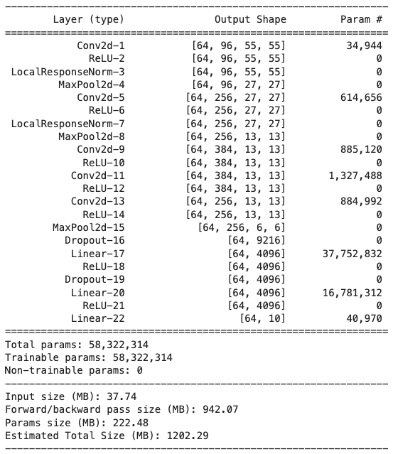
- Training
epochs = 20
l_ = []
pbar = trange(epochs)

for i in pbar:
    train_loss, correct, total, = 0.0, 0, 0

    for data in trainloader:
        images, labels = data[0].to(device), data[1].to(device)
        outputs = model(images)

        optimizer.zero_grad()
        loss = criterion(outputs, labels)
        loss.backward()
        optimizer.step()

        train_loss += loss.item()
        _, predicted = torch.max(outputs.detach(), 1)

        total += labels.size()[0]
        correct += (predicted == labels).sum().item()

    l = train_loss / len(trainloader)
    l_.append(l)
    acc = 100 * correct / total

    pbar.set_postfix({
        'loss' : l,
        'train acc' : acc
    })


print(l_)
성능이 잘 나오지 않아서 tr.Resize(128)로 바꿔서 진행했다. (cifar 데이터셋 이미지 크기가 32 x 32로 작은 편임)
그대신 아래와 같이 fc6을 바꿔줘야 한다.
self.fc6 = nn.Sequential(
            nn.Dropout(0.5),
            nn.Linear(1024, 4096),
            nn.ReLU(inplace=True),
        )
loss = 0.772, train accuracy : 74.3
- Testing
correct, total = 0, 0

with torch.no_grad():
    model.eval()
    test_loss = 0.0

    for data in testloader:
        images, labels = data[0].to(device), data[1].to(device)
        outputs = model(images)
        test_loss += loss.item()

        _, predicted = torch.max(outputs.data, axis=1)
        total += labels.size(0)
        correct += (predicted == labels).sum().item()

print(f"Test loss : {test_loss / len(testloader)}")
print(f"Accuracy : {correct / total:.2f}")
loss : 0.813, test accuracy : 71.80
'Artificial Intelligence > Papers' 카테고리의 다른 글
| [ 논문 구현 ] VGGNet 파이토치로 구현하기 (0) | 2024.08.15 |
|---|