1. 논문 소개
'Very Deep Convolutional Networks for Large-Scale Image Recognition'
Karen Simonyan, Andrew Zisserman (ICLR 2015)
(1) Abstract
- Convolution network 깊이가 large-scale image recognition에 미치는 영향에 대한 연구를 진행함
- 매우 작은 convolution filters (3 x 3)로 16 ~ 19 layers 아키텍처를 구성하여 상당한 성능 개선을 이룸
- 2014년 ILSVRC에서 1, 2위를 차지함
- 다른 데이터셋에서도 잘 일반화되어 sota 결과를 얻을 수 있었음
(2) Introduction
- ConvNet이 컴퓨터 비전 분야에서의 성능 향상에 도모하는 바가 커지면서, 2012년 AlexNet의 성능을 뛰어넘기 위한 노력을 많이 하고 있음
- 본 논문에서는 'depth'에 집중하기로 함. convolutional layer를 추가함으로써 점차 깊이를 증가시켜나간다.
(3) ConvNet Configurations
1) Architecture
- input : 224 x 224 RGB image (학습 데이터의 평균으로 빼주기)
- kernel : 3 x 3, stride : 1, padding : 1
- MaxPooling : 2 x 2, stride : 2
- FC layers : 4096 channels 2개, 마지막엔 1000-way (softmax layer)
- ReLU 사용
- LRN 사용 안 함 (오히려 그런 normalization이 성능 향상에 도움이 안 되었고, 메모리 소모와 연산 시간만 늘렸다고 함)
2) Configuration

- 깊이 11 (8 conv, 3 FC) ~ 깊이 19 (16 conv, 3 FC)

- 깊이에 따른 파라미터 개수인데, 크게 차이나지 않음
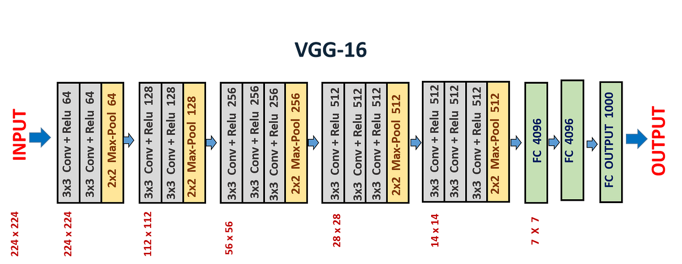
- VGG16 구조 도식화

3) Discussion
- VGGNet은 이전의 ILSVRC 대회에서 우수한 성능을 보인 모델들과의 상당한 차이가 있음
- 첫번째 conv layer뿐만 아니라 전체 네트워크에 걸쳐 3 x 3의 매우 작은 receptive field를 사용한다.
- 작은 receptive field을 사용하는 것의 이점?
1) 작은 kernel을 여러 개 사용하는 것과 큰 kernel 한 개를 사용하는 것이 동일한 크기의 피처맵을 얻을 수 있음
2) decision function을 더 discriminative하게 만들 수 있음
3) 더 적은 파라미터가 필요함
예) 2개의 3 x 3 커널을 사용하는 것과 1개의 5 x 5 커널은 동일한 크기의 피처맵 생성!

입력 채널, 출력 채널 모두 C개라고 가정하면,
- 2개의 3 x 3 커널 : 2 * (3 * 3 * C * C) = 18C*C
- 1개의 5 x 5 커널 : (5 * 5 * C * C) = 25C * C
2개의 3 x 3 커널의 파라미터보다 1개의 5 x 5 커널의 파라미터 개수가 더 많다.
- 1 x 1 conv. layers 사용 : receptive field에 영향을 주지 않으면서, non-linearity 증가시키기 위해서 사용 (by. ReLU)
- GoogLeNet도 small convolutional filters (1 x 1, 5 x 5, 3 x 3)를 사용했다는 점이 유사하지만, VGGNet 보다 훨씬 복잡하여 계산량이 어마어마하다.
(4) Classification Framework
1) Training
- Mini batch gradient descent (batch size : 256, momentum : 0.9)
- L2 regularization : $5 \cdot 10 ^{-4}$
- Dropout : 0.5
- 초기 learning rate : $10^{-2}$ → validation score 개선 없는 경우 10배 감소시킴 (총 3회 감소)
- 네트워크 가중치의 초기화가 중요하므로, 얕은 모델부터 학습 시작하고, 학습 중에 레이어가 변경될 수 있도록 했음
- Random Initialization은 정규 분포 상에서 weight를 샘플링했음 (평균 0, 표준편차 $10^{-2}$)
2) Testing
- 입력 이미지의 크기에서 training scale을 S, testing scale을 Q라고 했을 때, 둘이 서로 같을 필요는 없음
- input image 크기에 따라 variable spatial resolution을 출력하기 때문에, class score map을 'sum-pooled'을 통해 spatially average 한다.
2. Summary
- 네트워크의 깊이와 모델 성능 영향에 집중
- Convolution 커널 사이즈를 3 x 3으로 고정
- 커널 사이즈가 크면 이미지 사이즈 축소가 급격하게 이뤄져서 더 깊은 층을 만들기 어렵고, 파라미터 개수와 연산량도 더 많이 필요
- 여러 개의 3X3 Convolution 연산을 수행하는 것이 더 뛰어난 Feature 추출 효과를 나타냄
- 개별 Block내에서는 동일한 커널 크기와 Channel 개수를 적용하여 동일한 크기의 feature map들을 생성
- 이전 Block 내에 있는 Feature Map 대비 새로운 Block내에 Feature Map 크기는 2배로 줄어 들지만 채널 수는 2배로 늘어남 (맨 마지막 block 제외)
3. Code
!pip install torchsummary

import numpy as np
import pandas as pd
import os
import matplotlib.pyplot as plt

import torch
import torch.nn as nn
import torch.nn.functional as F
import torch.optim as optim

from torch.utils.data import DataLoader, Dataset, random_split
from torch.utils.data import random_split

from torchsummary import summary

import torchvision
from torchvision.utils import make_grid
import torchvision.transforms as tr

from tqdm import trange
# mean
tr_meanRGB = [ np.mean(x.numpy(), axis=(1, 2)) for x, _ in cifar10_tr ]
tr_meanR = np.mean([m[0] for m in tr_meanRGB])
tr_meanG = np.mean([m[1] for m in tr_meanRGB])
tr_meanB = np.mean([m[2] for m in tr_meanRGB])
# std
tr_stdRGB = [ np.std(x.numpy(), axis=(1, 2)) for x, _ in cifar10_tr ]
tr_stdR = np.std([m[0] for m in tr_stdRGB])
tr_stdG = np.std([m[1] for m in tr_stdRGB])
tr_stdB = np.std([m[2] for m in tr_stdRGB])
mean = [tr_meanR, tr_meanG, tr_meanB]
std = [tr_stdR, tr_stdG, tr_stdB]
tr_transform = tr.Compose([
tr.ToTensor(),
tr.Resize(128), # 크기 조정
tr.RandomHorizontalFlip(p=0.7),
tr.Normalize(mean=[0.49139965, 0.48215845, 0.4465309], std=[0.060528398, 0.061124973, 0.06764512])
])
te_transform = tr.Compose([
tr.ToTensor(),
tr.Resize(128), # 크기 조정
tr.Normalize(mean=[0.49139965, 0.48215845, 0.4465309], std=[0.060528398, 0.061124973, 0.06764512])
])tr_meanRGB, tr_stdRGB 값을 구해서 이후에는 직접 Normalize에 넣어주는 방식으로 진행했음.
torch.manual_seed(11)

cifar10_tr = torchvision.datasets.CIFAR10(root='./data', download=True, train=True, transform=tr_transform)

val_size = 10000
train_size = len(cifar10_tr) - val_size
cifar10_tr, cifar10_val = random_split(cifar10_tr, [train_size, val_size])

cifar10_te = torchvision.datasets.CIFAR10(root='./data', download=True, train=False, transform=te_transform)
train 데이터를 train, valid로 나누어주었고, random_split을 사용했음
trainloader = DataLoader(cifar10_tr, batch_size=64, shuffle=True)
valloader = DataLoader(cifar10_val, batch_size=64, shuffle=False)
testloader = DataLoader(cifar10_te, batch_size=64, shuffle=False)
train, valid, test 데이터셋을 데이터로더로 넣어주고,
시각화
for images, _ in trainloader:
    print('images.shape:', images.shape)

    plt.figure(figsize=(16,8))
    plt.axis('off')
    plt.imshow(make_grid(images, nrow=16).permute((1, 2, 0)))

    break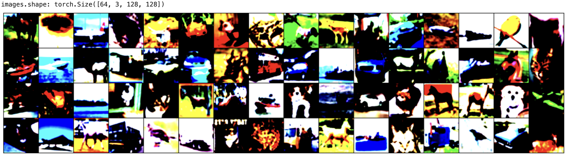
데이터 확인
images, labels = next(iter(trainloader))
print(labels)
print(images.shape, labels.shape)
VGGNet 모델 구현
device = torch.device('cuda:0' if torch.cuda.is_available() else 'cpu')

class VGGNet(nn.Module):

    def __init__(self, n_classes=10):
        super().__init__()

        self.conv1 = nn.Sequential(
            nn.Conv2d(3, 64, kernel_size=3, stride=1, padding=1),
            nn.ReLU(),
            nn.Conv2d(64, 64, kernel_size=3, stride=1, padding=1),
            nn.ReLU(),
            nn.MaxPool2d(2, 2)
        )

        self.conv2 = nn.Sequential(
            nn.Conv2d(64, 128, kernel_size=3, stride=1, padding=1),
            nn.ReLU(),
            nn.Conv2d(128, 128, kernel_size=3, stride=1, padding=1),
            nn.ReLU(),
            nn.MaxPool2d(2, 2)
        )

        self.conv3 = nn.Sequential(
            nn.Conv2d(128, 256, kernel_size=3, stride=1, padding=1),
            nn.ReLU(),
            nn.Conv2d(256, 256, kernel_size=3, stride=1, padding=1),
            nn.ReLU(),
            nn.MaxPool2d(2, 2)
        )

        self.conv4 = nn.Sequential(
            nn.Conv2d(256, 512, kernel_size=3, stride=1, padding=1),
            nn.ReLU(),
            nn.Conv2d(512, 512, kernel_size=3, stride=1, padding=1),
            nn.ReLU(),
            nn.MaxPool2d(2, 2)
        )

        self.conv5 = nn.Sequential(
            nn.Conv2d(512, 512, kernel_size=3, stride=1, padding=1),
            nn.ReLU(),
            nn.Conv2d(512, 512, kernel_size=3, stride=1, padding=1),
            nn.ReLU(),
            nn.MaxPool2d(2, 2)
        )

        self.fc6 = nn.Sequential(
            nn.Dropout(0.5),
            nn.Linear(512*4*4, 4096),
            nn.ReLU(),
        )

        self.fc7 = nn.Sequential(
            nn.Dropout(0.5),
            nn.Linear(4096,4096),
            nn.ReLU(),
        )

        self.fc8 = nn.Sequential(
            nn.Linear(4096, n_classes),
        )

    def forward(self, x):
        x = self.conv1(x)
        x = self.conv2(x)
        x = self.conv3(x)
        x = self.conv4(x)
        x = self.conv5(x)
        x = x.view(x.size(0), -1)
        x = self.fc6(x)
        x = self.fc7(x)
        x = self.fc8(x)

        return x
학습 준비
model = VGGNet().to(device)
criterion = nn.CrossEntropyLoss()

optimizer = optim.Adam(model.parameters(), lr=1e-3, weight_decay=1e-4)
scheduler = optim.lr_scheduler.ReduceLROnPlateau(optimizer, mode='min', factor=0.1, patience=5, verbose=True)

# early stopping
early_stopping_epochs = 5
best_loss = float('inf')
early_stop_counter = 0

summary(model, input_size=(3, 128, 128))
PyTorch에서는 early stopping을 제공하고 있지 않기 때문에, 직접 구현해주었음
학습
epochs = 30

for epoch in range(epochs):
    model.train()
    train_loss, correct, total = 0.0, 0, 0

    # Train
    for data in trainloader:
        images, labels = data[0].to(device), data[1].to(device)

        outputs = model(images)

        optimizer.zero_grad()
        loss = criterion(outputs, labels)
        loss.backward()
        optimizer.step()

        train_loss += loss.item()
        predicted = torch.argmax(outputs, 1)

        total += labels.size()[0]
        correct += (predicted == labels).sum().item()

    print(f'Epoch [{epoch+1}/{epochs}] || Loss:{train_loss / len(trainloader)} || Accuracy:{100 * correct / total}')


    # Valid
    model.eval()
    valid_loss = 0.0

    for data in valloader:
        images, labels = data[0].to(device), data[1].to(device)
        outputs = model(images)
        loss = criterion(outputs, labels)
        valid_loss += loss.item()

    if valid_loss > best_loss:
        early_stop_counter += 1
    else:
        best_loss = valid_loss
        early_stop_counter = 0

    if early_stop_counter >= early_stopping_epochs:
        print("Early Stopping!")
        break
Test
correct, total = 0, 0

with torch.no_grad():
    model.eval()
    test_loss = 0.0

    for data in testloader:
        images, labels = data[0].to(device), data[1].to(device)
        outputs = model(images)
        test_loss += loss.item()

        _, predicted = torch.max(outputs.data, axis=1)
        total += labels.size(0)
        correct += (predicted == labels).sum().item()

print(f"Test loss : {test_loss / len(testloader)}")
print(f"Accuracy : {correct / total:.2f}")'Artificial Intelligence > Papers' 카테고리의 다른 글
| [ 논문 구현 ] AlexNet 파이토치로 구현하기 (0) | 2024.08.05 |
|---|